Hydrological Theory

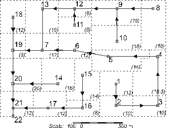
Rainfall-runoff simulation requires certain assumptions with respect to the level of discretization to be employed and the parameter values to be used for the sub-areas.  When modelling very large watersheds a compromise is necessary between using sub-areas that are too small or too large.  Small sub-catchments impose cost penalties in data preparation and computation effort.  Large areas present problems in assigning values to parameters – such as overland flow length - that are a reasonable representation of the physical system.

The ratio of channel travel time to sub-area response time varies widely for areas that are close to or distant from the outflow point.  This variation results in a diffusion of the flow peaks from individual areas and accounts for a significant part of the basin lag.  In large catchments this basin lag can equal or exceed the overland flow travel time and attempts to represent this by distorting overland flow parameters are subjective, unrealistic and storm specific.  The process can be better represented by convoluting the overland flow response function with the derivative of the time-area diagram for the total watershed.  The resulting modified response function can then be convoluted with the effective rainfall to yield a good approximation to the runoff hydrograph for the total area.

Numerical experiments suggest that the unwieldy process of double convolution can be approximated by using a single convolution of overland flow and rainfall and then routing the resulting hydrograph through a hypothetical linear channel and linear reservoir.  The latter have lag times that are related to the maximum conduit travel time through the drainage network.  MIDUSS uses some preliminary guidelines to estimate the lags and partially automate the process.

This section describes the process used and compares a typical example with a fully discretized simulation.  It must be emphasized that the suggested method is preliminary and would benefit from further testing of either real or idealized cases to verify or improve the guidelines.

Example of a Large Catchment

The process is described with reference to the catchment area in Figure 7-27.  The runoff obtained from the discretized version will be compared to the approximate 'lumped-parameter’ version.  In Figure 7-27 the area in hectares of the sub-areas is shown in italics and in parenthesis in the lower-right corner of each rectangular area. 

Figure 7-27 – Discretized version of a large catchment
(Areas shown in hectares as (12) in lower right corners)

The system is subjected to a 5-year storm represented by a 360 minute Chicago hyetograph with a total depth of 50.45 mm (the MIDUSS default values).  All the sub-areas are assumed to have the same overland flow characteristics with the exception of area, i.e.

                Overland flow length           =              45 m

                Overland slope                     =              2.0 %

                Percent impervious              =              30 %

                Pervious roughness n         =              0.25

                Impervious roughness n     =              0.013

With this simplifying assumption, the response functions of the sub-areas will have the same time parameters and vary only with respect to the area.  Thus, for a triangular response function:

The drainage network is composed of pipes with a gradient of approximately 0.4%.  The output file from the discretized simulation is called ‘Large1.out’ and can be found in the ..\Samples\ folder of the Miduss98 directory.

The distribution of areas relative to the outflow point can be represented by a time-area diagram as illustrated in Figure 7‑ 28.  From Figure 7-27 you will note the rather circuitous (and unrealistic) drainage path of areas 1, 2 and 3.  This gives rise to the late contribution of the furthest upstream 32 ha which in turn makes the Time-Area diagram depart from the reasonably linear shape which is apparent over the first 15 minutes.  This feature makes the approximation more challenging.

Figure 7-28 – Time-Area diagram for the catchment of Figure 7-27

The time to equilibrium Te is 23.21 minutes from node #1 to the outflow point at node #22.  This is the time at which the entire catchment is contributing and is a function of the drainage network.  The time of concentration tc and therefore the timebase tb of the response function, is a characteristic of the overland flow.  Both quantities are also dependent on the magnitude of the storm.

The relative magnitude of Te and tc is an important parameter in determining the limit for lumped representation of a catchment.  If Te / tc << 1.0 then it is likely that overland flow dominates the runoff process and thus the overland flow response function is a reasonable approximation for the entire catchment.  In large catchments, Te / tc is larger (although still probably less than 1.0) and channel/pipe routing will play an important role in determining the shape and peak of the runoff hydrograph.

Combining Overland Flow and Drainage Network Routing

The combined effect of overland flow routing and drainage network routing can be obtained by convoluting one response function with the other.  The right side of Figure 7-29 shows a triangular response function being convoluted with the derivative of the time-area diagram to produce a modified response function.  This is then convoluted with the hyetograph of effective rainfall to produce the modified runoff hydrograph in the lower right corner of the figure. 

The unwieldy process of double convolution can be approximated by the process shown on the left side of the Figure 7-29.  The normal overland flow response function is convoluted with the effective rainfall to produce a ‘lumped’ runoff hydrograph.  This assumes that all the sub-areas contribute to runoff simultaneously.  This is then routed through a linear channel and linear reservoir.  If appropriate values can be set for Kch and Kres the resulting hydrograph should be a close approximation of the modified runoff hydrograph.

Figure 7-29 – Representation of the Lag and Route method

The total lag Ktot is defined as the sum of the two components Kch and Kres, i.e.

The distribution of the total lag between the two constituent parts is defined by a fraction  r  (0.0  <  r  <  1.0) as follows.

and

Estimating the Lag Values

Results from a limited number of numerical experiments suggest that some correlation exists between:

·         The total lag Ktot and the ratio of time to equilibrium to time of concentration (Te/tc), and

·         The fraction r = Kres/Ktot and the basin time to equilibrium Te

As preliminary guidelines the following relationships are used in MIDUSS.

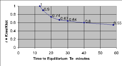
Values for the fraction r = Kres/Ktot are based on a curve which – for the data analyzed – approaches an asymptotic value of about 0.55 as shown in Figure 7-30.

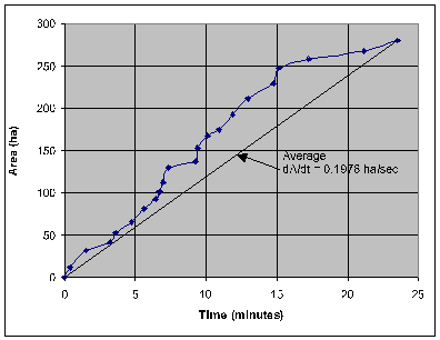
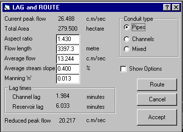
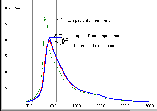
Figure 7-30 – Empirical curve defining r = Kres/Ktot = f(Te)

The data of Figure 7-30 is contained in a small data file called ‘LagRout1.dat’ which resides in the Miduss98 folder.  This file can be edited or updated as and when further numerical experimental results are available.  The trends suggested are interesting but inconclusive.  More experiments are required to test the sensitivity of the identified parameters to factors such as:

·         Shape and duration of storm

·         Size and shape of the catchment

·         Choice of overland routing model

·         The rainfall loss model employed.

Until such time as further test results are available you should use this feature with caution.  When possible, it is useful to carry out a comparison between the Lag and Route approximation and a typical discretized simulation to provide a measure of confidence in the method.  The next section describes the results obtained for the catchment of Figure 7-27.

Comparison of Discretized and Approximate Results

Refer to the output file …\MIDUSS\Samples\Large1.out  for details of the test described here. 

The fully discretized simulation produced a peak runoff of 19.136 c.m/s. 

The lumped catchment runoff is found to have a peak of 26.488 c.m/s

The Lag and Route command is then used with MIDUSS default values for all quantities with the exception of the catchment area aspect ratio which is set at 2000m/1400 m or 1.43 and the average pipe slope of 0.4%.  The form is shown in Figure 7-31 below.  The longest drainage path estimated by MIDUSS is 3397 m whereas scaling the reach from node #1 the length is 3900 m.  The underestimate is close to 13% and is due to the circuitous route from node #1 to node #5.  The error will result in a slightly higher peak flow for the reduced peak flow that is shown as 20.217 c.m/s.  A graphical comparison of the results is shown in Figure 7-32.  Apart from the over-estimated peak flow the approximation is reasonable.

If the Stream length is entered as 3900 m as a result of scaling the drawing (Figure 7_27) the result is improved.  The peak of the approximate runoff is reduced to 19.745 c.m/s with no measurable change in the general agreement between the discretized and approximate runoff hydrographs.  The effect of the change in stream length is summarized in the Table below.

By checking the output file you will also see that continuity is respected and the total runoff volume is given as 6.2605 ha-m in all cases.

You can experiment with this example by running the file ‘Large1.out’ in automatic mode.  After generating the database Miduss.Mdb, navigate to the Hydrograph/Start new tributary command following completion of the discretized simulation.  Change the command from ‘40’ to ‘- 40’ and then use the [RUN] button in the Automatic Control Panel to run up to that point.  You can then step through the ‘lumped’ runoff calculation and the Lag and Route approximation using the [EDIT] command button or in Manual mode

Figure 7-31 – Using the Lag and Route command

Figure 7-32 – Comparison of the Lag and Route approximation with the discretized runoff.

(c) Copyright 1984-2023 Alan A. Smith Inc.
Terms and Conditions       Privacy Policy