Theory - Calculating Runoff - SWMM

Hydrological Theory

Calculating Runoff

SWMM - RUNOFF Algorithm

From the MIDUSS Version 2 Reference Manual - Chapter 7
(c) Copyright Alan A. Smith Inc.

Figure 7-22 - Representation of the SWMM/RUNOFF algorithm.

The U.S. EPA SWMM model is made up of a number of large program modules. One of these - the RUNOFF block - is used to generate the runoff hydrograph from a sub-catchment. In MIDUSS, the ‘SWMM Method’ option uses a similar algorithm with the limitation that only the Horton or Green and Ampt infiltration equations are supported.

The method employs the surface water budget approach and may be visualized as shown in Figure 7-22. The incident rainfall intensity is the input to the control volume on the surface of the plane; the output is a combination of the runoff Q and the infiltration f. Considering a unit breadth of the catchment the continuity and dynamic equations which have to be solved are as shown in equations [7-44] and [7-45].

where L = overland flow length

B = catchment breadth

CM = 1.0 for metric units

1.49 for Imperial or US customary units

n = Manning roughness coefficient

y_d = surface depression storage depth

Rewriting [7-44] with q = Q/B and then substituting for Q by means of [7-45] yields the single equation:

If the depth on the plane at the start and finish of the time step Dt is represented by y₁ and y₂ respectively an equation for y₂ can be developed using the following approximations.

for y>0

Equations [7-47] ‑ [7-49] are solved using a Newton Raphson method to yield a solution for y2 which is then used to obtain a value for Q.

It can be shown (Smith, 1986a, see references) that the algorithm developed above is equivalent to convoluting the storm rainfall with a Dirac d-function and then routing the resulting 'instantaneous' runoff through a nonlinear reservoir with storage characteristics given by:

where

In equation [7-50] 'A' is the catchment drainage area and other terms are as defined previously (see equations [7-41] and [7-45]).

Three points of some significance arise with respect to the ‘SWMM Method’ option.

(1) Considering the method to be equivalent to routing the instantaneous runoff through a nonlinear reservoir, it follows that the peak of the outflow must lie on the recession limb of the inflow. Consequently the time to peak for pervious and impervious fractions will not differ significantly and the total runoff will not exhibit the double peaked hydrographs which are sometimes encountered with the ‘Rectangular’ or ‘Triangular SCS’ options.

(2) The form of equations [7-44] and [7-45] implicitly assumes that the depth of flow over the plane is quasi-uniform. This over-estimates the volume on the plane and will usually result in over-attenuation of the peak runoff.

(3) Since infiltration is assumed to continue over the entire surface after cessation of rainfall as long as the average depth is finite, the recession limb of the runoff hydrograph will generally be much steeper than for the ‘Rectangular’ or ‘Triangular SCS’ options. In practice, after cessation of rainfall, the surface water tends to concentrate in pools and rivulets so that the area over which the infiltration continues is likely to be much less than the total area A. A more realistic representation of the infiltration after the storm is likely to be intermediate between the two extreme cases represented by the ‘SWMM Method’ method on one hand and the ‘Triangular SCS’ or ‘Rectangular’ method which employs the concept of effective rainfall. This feature is sufficiently important that a detailed example is presented in the following section in order to illustrate the fundamental difference between the methods.

An Example of the SWMM Runoff Algorithm

The object of this example is to compare the overland flow that is generated by the ‘SWMM Method’ option with that which would be obtained using an effective rainfall approach. For simplicity we shall assume a catchment of 5.0 ha with no impervious area and no depression surface storage. The storm used is a 3rd quartile Huff storm with a total rainfall depth of 30 mm occurring in 60 minutes. Infiltration will be modelled by the Horton method with the following parameter values:

· n = 0.25

· f0 = 40 mm/hour

· fc = 20 mm/hour

· K = 0.25 hours

· y_d = 0

To simulate the SWMM algorithm using an effective rainfall approach we shall make use of equation [7.50] to define a nonlinear reservoir through which the instantaneous runoff is routed. This hydrograph can be created by convoluting the effective rainfall with an impulse (also known as a Dirac d-function) which can be simulated by specifying a very short overland flow length.

The steps are summarized as follows. You may find it instructive to run this example on your own computer as you read through the steps.

· In the Time Parameters use 2 minute timesteps and a storm duration of 60 minutes.

· Define the Huff storm; use 30 mm rainfall; 60 minutes duration; 3rd quartile.

· The impervious characteristics are not important but we must use the Horton method. Set n = 0.015 and the other parameters to zero.

· The first catchment 101 is used to represent the Dirac d-function so use the following parameters.

Area = 5.0 ha

Length = 0.1 m

Slope = 2.0 %

Percent impervious = 0

For the infiltration parameters use the Horton method with:

fo = 40 mm/hour

fc = 20 mm/hour

K = 0.25 hour

yd = 0

The peak effective rainfall intensity is found to be 68.279 mm/h. Use the ‘Rectangular’ option since this most closely approximates an impulse. The peak runoff is 0.948 c.m/s. A few seconds with a calculator will confirm that for an area of 5 hectares this is equivalent to 68.279 mm/h.

Figure 7-23 – Statistics of the Dirac-d response hydrograph

· We want to route this runoff through an imaginary pond with stage discharge characteristics as given by [7‑ 50]. Use the Hydrology/Add Runoff command to define the inflow to the pond to be used in step (7).

· The final step to simulate the SWMM hydrograph is by routing the instantaneous runoff through a nonlinear reservoir. For the data used in this example, the value of C in equation [7-50] works out to be 1115.39. We now define a pond with discharges ranging from 0.0 to 0.25 in increments of 0.025 - i.e. 11 stages. Figure 7-25 shows the result of a pond design. The value of each storage volume is given by 1115.39 x Q^0.6. The peak outflow is found to 0.246 c.m/s In Figure 7-25, the hydrograph has been extended to 130 minutes.

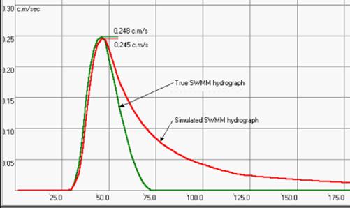
Figure 7-24 ‑ Design of a hypothetical pond.

· The next step is to generate the ‘SWMM method’ hydrograph, so define another catchment with the same parameters as in step (4) but with a flow length of 50 m. The infiltration options are the same as before. The peak runoff is found to be 0.248 c.m/s.

The similarity in peak flows is promising, but the true test is to compare the plotted hydrographs. Figure 7-24 shows the ‘SWMM Method’ and simulated SWMM hydrographs

The rising limbs of the two hydrographs are in good agreement apart from a slight lag of about 2 minutes which is the shortest 'impulse' that MIDUSS can create when Dt is 2 minutes. However, immediately following the cessation of the effective rainfall the ‘SWMM Method’ recession limb drops more steeply. This is due to the fact that the surface water budget method assumes that infiltration continues as long as there is excess water on the pervious surface whereas the effective rainfall approach - which produced the longer curve in Figure 7-25 - assumes that infiltration stops at the end of the effective rainfall. The two recession limbs start to diverge at t = 50 min. which marks the end of the effective rainfall hyetograph.

Figure 7-25 ‑ Comparing the SWM HYD and simulated SWMM hydrographs.

Figure 7-26 ‑ Statistics of the ‘SWMM Method’ hydrograph.

This difference serves also to explain the anomaly that appears in the hydrograph statistics screen when using ‘SWMM Method’ option. Figure 7-26 shows the summary statistics obtained at the end of step (7) and you will note that the runoff volume (296.2 c.m) is much less than that for the effective rainfall volume of 636.38 c.m. (from Figure 7-23).

This may not always be the case and you should repeat this experiment with a finite value for depression surface storage - say 2 mm or 100 c.m over the 5 hectares of area. You will find that the effective rainfall volume is reduced by exactly 100 c.m. The infiltration and runoff volume are also reduced by amounts which add up to 100.0 c.m. less the volume still trapped in surface depressions when the calculation was ended. If continued long enough, this too would have infiltrated thus balancing the books properly. Hence the name 'surface water budget'.