|
|
|


Hydrological Theory
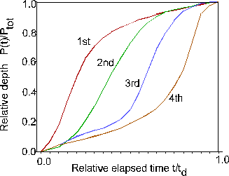
Based on data from watersheds in the mid-western USA, Huff (see References) suggested a family of non-dimensional, storm distribution patterns. The events were divided into four groups in which the peak rainfall intensity occurs in the first, second, third or fourth quarter of the storm duration. Within each group the distribution was plotted for different probabilities of occurrence. MIDUSS uses the median curve for each of the four quartile distributions. The non-dimensional curves are illustrated in Figure 7-3 below and are tabulated in Table 7-1.
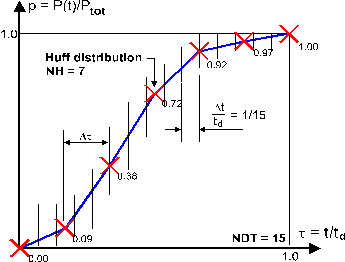
Figure 7-3 - Huff's four storm distributions. To define a storm of this type you must provide values for the total depth of rainfall (in millimetres or inches), the duration of the storm (in minutes) and the quartile distribution required (i.e. 1, 2, 3 or 4). The duration must not exceed the maximum storm duration defined in the Hydrology/Time parameters menu command and, as with the Chicago storm option, an error message is displayed if this constraint is violated. Once the parameter values have been entered and confirmed by pressing the [Display] command button, the hyetograph is displayed in both graphical and tabular form. You can experiment by altering any of the data - even the type of storm - and re-using the [Display] button until you press the [Accept] button to save the storm and close the Storm command. The four quartile Huff distributions are approximated by a series of chords joining points defined by the non-dimensional values in the table referenced below. Figure 7-4 shows a typical curve (not to scale) which for clarity uses only a very small number of steps. The time base for the NH dimensionless points defining the ‘curve’ is subdivided into dimensionless time steps defined by:
where NH = number of points defining the Huff curve (shown as NH = 7 but usually much more) NDT = number of rainfall intensities required (shown as only 15 in Figure 7-4).
Figure 7-4 - Discretization of a Huff curve. The values of the dimensionless fractions Pk and Pk+1 at the start and finish of each time-step are obtained by linear interpolation and the corresponding rainfall intensity is then given as:
where
For the example shown in Figure 7-4, the Huff 2nd quartile curve is approximated by NH=7 points with a storm duration which is divided into 15 time steps. Then Dt = (7-1)/15 = 0.4. The calculation of the rainfall fractions Pk+1 required for eq. [7.10] is then carried out as shown in the table below.
Table 1 - P(t)/Ptot for Four Huff Quartiles t/td P(t)/Ptot for quartile 1st 2nd 3rd 4th 0.00 0.000 0.000 0.000 0.000 0.05 0.063 0.015 0.020 0.020 0.10 0.178 0.031 0.040 0.040 0.15 0.333 0.070 0.072 0.055 0.20 0.500 0.125 0.100 0.070 0.25 0.620 0.208 0.122 0.085 0.30 0.705 0.305 0.140 0.100 0.35 0.760 0.420 0.155 0.115 0.40 0.798 0.525 0.180 0.135 0.45 0.830 0.630 0.215 0.155 0.50 0.855 0.725 0.280 0.185 0.55 0.880 0.805 0.395 0.215 0.60 0.898 0.860 0.535 0.245 0.65 0.915 0.900 0.690 0.290 0.70 0.930 0.930 0.790 0.350 0.75 0.944 0.948 0.875 0.435 0.80 0.958 0.962 0.935 0.545 0.85 0.971 0.974 0.965 0.740 0.90 0.983 0.985 0.985 0.920 0.95 0.994 0.993 0.995 0.975 1.00 1.000 1.000 1.000 1.000
|
|||||||||||||||||||||||||||||||||||||||||||||||||||||
|
|
|||||||||||||||||||||||||||||||||||||||||||||||||||||
|
(c) Copyright 1984-2023 Alan A. Smith Inc. |
|
|