Tools

• IDF Curve Fit: Computes Chicago storm parameters ‘a’, ‘b’ & ‘c’ for observed data.

• Time of Concentration: Estimates the time of concentration at various locations in the drainage network.

• Roughness Height: Converts roughness element height to a Manning 'n’ value.

• Edit Storm: Lets you modify an existing Mass Rainfall Curves file or create a new one.

IDF Curve Fit

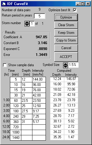
The IDF Curve Fit tool manipulates data describing an Intensity-Duration-Frequency relates for a particular geographical locality and can be used in two modes:

1. To compute the ‘a’, ‘b’ and ‘c’ parameters of a Chicago hyetograph that most closely approximates a set of observed rainfall data.

2. To compute the IDF curve for user-supplied values of the three coefficients and compare this with observed data.

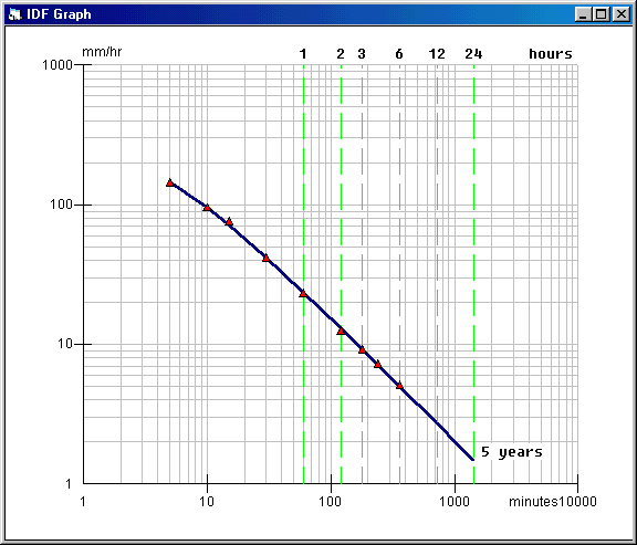
The mode is selected by checking the ‘Optimize’ check box on the form or clearing it to simply compute the curve for specified values of ‘a’, ‘b’ and ‘c’. 

The above display shows data that has been entered for the first “Optimize’ mode of operation.  In the grid on the left for Time, Depth and Intensity a column of time intervals is displayed as shown.  These values can be customized if desired.

For any time interval the rainfall can be defined either as a total depth of rainfall or as an average intensity over the time interval. Entering either value automatically calculates and displays the other. The number of data pairs is automatically displayed in the top of the form and not every time interval need be entered.

When the [Optimize] button is clicked several pieces of information are displayed:

• The optimal values of the three parameters

• The computed values of Depth and Intensity for each time interval. These are shown in the right hand grid.

• A ‘log-log’ graph of both observed and computed values is displayed. A typical result is shown below.

Time of Concentration

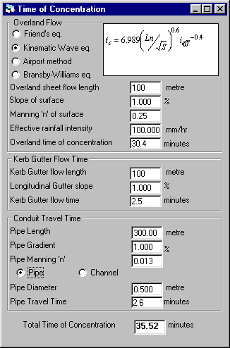
With few exceptions, peak runoff will occur when the entire catchment area is contributing to the outflow. Thus the storm duration should be long enough for the runoff from the most remote area – in terms of time of travel – to reach the outflow point. This is commonly referred to as the Time of Concentration Tc.

The time of concentration is calculated as the sum of up to three components of travel time. These are:

• Flood wave travel time of overland flow

• Travel time in relatively small collector channels or gutters

• Travel time in a storm conduit such as a circular pipe or a channel of general trapezoidal cross-section.

For the overland flow you can select either the Friend’s equation or the Kinematic equation.

Each of the three components requires entry of data to describe the length, gradient and roughness of the conduit or surface. In addition, overland flow may also depend on the intensity of the effective rainfall.

On entry of a finite length, the time is computed for each component and the total is displayed as the Time of Concentration. If required, one or two of the flow components can be ignored by entering a zero length in the appropriate data field for length.

Roughness Height

MIDUSS design routines use the Manning ‘n’ to describe surface roughness. Users who prefer to define roughness in terms of the equivalent roughness height can use the Roughness Height tool to convert from roughness height to Manning ‘n’. Once calculated, the computed value can be imported into the next design command by clicking the [Use for Design] button.

Edit Storm

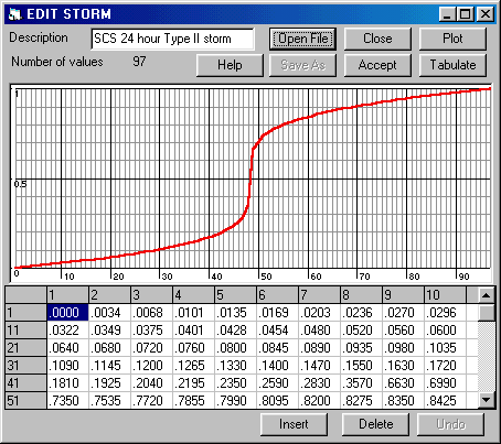
One of the options in the Storm command is to use a pre-defined curve known as a Mass Rainfall Distribution curve. These files are given the extension *.MRD and define the fraction of rainfall depth R(t)/ Rtot as a function of the ratio of elapsed time over total storm duration. Typical examples are the various Huff storm quartiles and the SCS hyetographs.  The Edit Storm Tool lets you edit or create MRD files.

The values can be edited by graphical manipulation or numerically.

Graphical Edits Position the mouse pointer on one of the vertical grid lines and either
above or below the red line. Each mouse click causes the numerical value in the table to increase or decrease by 0.01 and the plotted red curve shows the change.

Numerical Edits Click on any cell in the grid with the exception of the 0.0 and 1.0
values and type in the desired value. Any change in either the graphical or tabular display is reflected in the other. The array of values must start with zero and end with 1.0 and the intermediate values must increase monotonically.
 

(c) Copyright 1984-2023 Alan A. Smith Inc.
Terms and Conditions       Privacy Policy